A Primer on Current & Past Deep Learning Methods for NLP
Before You Read:
This article is the first of two that I will publish. This post serves to provide info on current & past deep learning methods for NLP tasks. This information is useful for understanding the second article, which will be about the novel Adapter architecture. As a disclaimer, this article serves solely to inform and will not be a guide for the implementation of the methods presented.
This post assumes a basic knowledge of machine learning concepts and is intended for those who are interested in the NLP space. This post starts from neural networks and conceptually summarizes the different improvements to NLP models up until the transformer model.
Background: Neural Networks
A neural network learns a generalized mapping or a function relating some input to output(s) for any relevant task. An example task could be learning a sentence’s sentiment or identifying objects in an image. To leverage neural networks, the task must represent its inputs and outputs as numerical values. At its core, a neural network is constructed of a series of linear and non-linear layers that successively transform the input to the output. The parameters in these layers are “learned” so that the final output of a neural network matches the true labels in a training dataset as closely as possible while also generalizing on unseen datasets. In the process of “learning,” the parameters are optimized for the lowest error on the training data and verified later on unseen test data. The gradient of the error to be minimized relative to each parameter provides the direction in which the parameter should be updated to reduce error. In a supervised setting, this procedure is repeated over the training dataset (often in multiple mini-batches) to optimize stochastically. This is a common procedure for using neural nets for any general task.
Tasks differ in their input type (e.g., images, sentences, audio waveforms, video). Different neural network architectures have evolved to exploit the inputs and their dependencies. In the case of object detection, convolution neural networks (CNNs) learn image processing filters that identify relevant patterns in a set of images to accurately identify one or more target objects.
In the above example, we are dealing with a fixed-length input. However, in the case of natural language processing, the input length could vary (e.g., by the number of words), and the sequence in which the words are said matters. For example, “I had my car cleaned” has a different meaning from “I had cleaned my car” despite using the same words (English Language Learners Stack Exchange, “Grammar — Changing the Word Order Changes the Meaning?”). This situation requires a neural network architecture that can handle an unspecified number of inputs and be sensitive to the order in which they appear.
Recurrent neural networks maintain a hidden state and learn an update function to update the hidden state based on the next input in the sequence. In this manner, a single update function can be learned that updates the hidden state at each time step in a sequence, processing the next input in the sequence until the end. The hidden state at the conclusion of the sequence will be relevant to completing the task at hand.
Recurrent Neural Networks
Sequential information is preserved in the recurrent network’s hidden state, which spans many time steps as it cascades forward, and impacts the processing of each new sample. This is important because there is information in the sequence itself: correlations are identified between events. “Long term dependencies” refers to the idea that “an event downstream in time depends upon, and is a function of, one or more events that came before” (Pathmind, “A Beginner’s Guide to LSTMs and Recurrent Neural Networks”).
To illustrate the mechanics, Figure 1 shows an RNN (blue box) applied at each time step. At each time step, you are retrieving the next part of the input and combining it with the current hidden state to generate a part of the output at that time step and feeding it to the RNN. This produces part of the output for the next time period as well as an updated hidden state. At any point in time, you have an output sequence and an output hidden state. At the end of the sequence, the output hidden state can be used as a feature vector to prime any other learning task.

An RNN can “simultaneously take a sequence of inputs and produce a sequence of outputs… [which is useful] for predicting time series such as stock prices: you feed it prices over the last N days and it must output the prices shifted by one day into the future” (O’Reilly, “Chapter 4: Recurrent Neural Networks). In the stock price example, a sequence of inputs (stock prices over the last N days) is utilized to produce a sequence of outputs (from N-1 days ago to tomorrow). This is shown in the top-left of figure 2 below.
Let’s say that you feed the network a sequence of inputs and ignore all outputs asides from the final one, as shown in the top-right of figure 2 below. This would be a sequence-to-vector network. This is different from the previously described network because rather than returning each output of the input sequence, only the last output is returned. For example, sentiment analysis takes the review (text data: a sequence of words) as input and outputs a vector with the identified sentiment (e.g., a sentiment score on a scale from negative (-1) to positive (+1) of the review as a whole).
The bottom-left picture in figure 2 shows a vector-to-sequence network. This involves feeding the network a single input at the first time step and outputting a sequence. An example would be image captioning: the input is an image and the output is a caption (a sequence of words) for the image.
Finally, the bottom-right image showcases the two-step, encoder-decoder model, which will come up when discussing Transformers later in this post. In the encoder-decoder model, you could have a sequence-to-vector network (encoder) followed by a vector-to-sequence network (decoder). A good example of the encoder-decoder model is language translation. An input sentence in a source language is converted by the encoder to a single vector representation which is decoded by the decoder to a sentence in a target language. This method is preferable to simply using a single sequence-to-sequence network because the last words in a sentence can impact the first words of the translation (O’Reilly, “Chapter 4: Recurrent Neural Networks).

When training a vanilla RNN on long sequences, you’ll need to run it over many time steps, which makes the RNN an extremely deep network. This presents two problems (that aren’t specific to RNNs but rather a generalization of any deep neural network): (1) vanishing/exploding gradients and (2) long training times. While there are techniques to alleviate these issues (e.g., batch normalization, nonsaturating activation functions, gradient clipping, etc.), the training will still be slow for RNNs when handling long sequences.
A common workaround to the above is to unroll the RNN over a limited number of time steps during training in a process called truncated backpropagation through time. However, this method prevents the model from learning long-term patterns (O’Reilly, “Chapter 4: Recurrent Neural Networks). Handling long sequences is crucial because significant events much earlier in the sequence could have a lasting influence on the output many time steps later (e.g., a negation at the beginning of a sentence or the result of a presidential election when analyzing political data).

RNNs are trained by backpropagating error using gradients through layers (time). Each layer corresponds to an update function that is applied at every time step. As you chain functions together for forward propagation, backward propagation multiplies their gradients (chain rule); the longer the chain, the more gradient terms that are multiplied together. Depending on the norm (magnitude) of the gradients multiplied, this product could become unstable. As a result, for deep networks, the norm can either go to zero (vanishing gradient — difficult to learn long-term dependencies) or go to infinity (exploding gradient — the value becomes NaN) exponentially fast.

We now understand that long-running sequences allow for vanishing and exploding gradients, both of which make learning in RNNs difficult. Therefore, one of the criteria for learning is stable gradients. Limiting the influence of the input length isn’t ideal because it prevents learning long-term dependencies in the input, which are sometimes critical. Instead, vanilla RNNs were improved by introducing memory that extended over the long and short term in an LSTM module — an architecture developed in 1997.
Long Short-term Memory Units
LSTMs introduced a long-short term memory cell that has a branch that lets past information skip a lot of processing and move on to the next layer (i.e., memory is retained for longer sequences). This enables the long-term dependencies to propagate directly without relying on intermediate layers. This is similar to the concept of memory, where relevant information for the future can be stored to be directly retrieved. LSTMs introduce memory cells that have a dynamic state which is accessible to each time period (each time period accesses the current state). Information in the cell state is managed via special neurons called “gates,” which control updating and forgetting information (i.e., what is stored in memory and for how long). A great example of the LSTM’s ability to retain memory over a vanilla RNN is below.

LSTMs have a memory cell state, which is the topmost line in figure 6. It goes through a few linear interactions but info can pass through it unchanged. The LSTM can remove or add information to the cell state through “gates” that optionally leave information unchanged over time. The LSTM has three important gates: (1) forget gate: decides what information from previous inputs to forget; (2) input gate: decide what new information to remember; (3) output gate: decide which part of the cell state to output (Quora, “What Is the Downside of Using LSTM versus RNN in Deep Learning?”). These gates have learnable parameters that enable it to learn what information that is task-relevant to retain or forget over the input sequence. An example of this could be retaining the gender of a subject in a sentence or a negation at the beginning of a sentence. In summary, LSTMs learn to recognize an important input (as facilitated by the input gate), store it in the long-term state, preserve it for as long as necessary (forget gate), and extract info when necessary (O’Reilly, “Chapter 4: Recurrent Neural Networks).
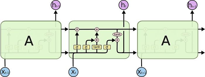
It’s important to mention that there are many variations of LSTMs. One example is an LSTM with “peephole connections,” which let gate layers look at cell state. Another example is coupled forget and input gates that couple the decision to add or forget information (forget only happens when there is an input in its place; new values are input only when something older is forgotten). A popular variant is the Gated Recurrent Unit (GRU) that combines the forget and input gates into an “update gate” and merges the cell state and hidden state. It is simpler than vanilla LSTMs (“Understanding LSTM Networks — Colah’s Blog”). This is a small sample of existing variants.
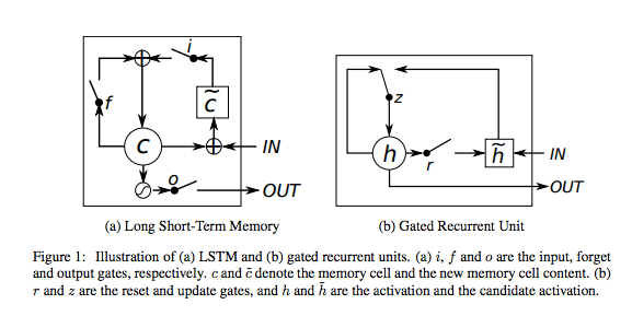
While vanilla RNNs are slow, LSTMs are even slower and harder to train (due to complexity and hyperparameter tuning). Input data for both methods still need to be passed sequentially (the input of the previous state needs to be given to make the next operation possible). Because modern-day GPUs utilize parallelization, processing data sequentially is inefficient (CodeEmporium, Transformer Neural Networks — EXPLAINED! (Attention Is All You Need)). Transformers address this inefficiency well.
Additionally, while memory is helpful for carrying information efficiently over long sequences, deciding how much weight should be given to that information is a separate concern. This requires the mechanism of attention and vanilla RNNs were introduced to the concept of attention (where a model can learn to make predictions by selectively attending to a given set of data), which have been adopted in other neural network architectures as well.
The Attention Mechanism
In 2017, the Transformer neural network architecture was introduced. With Transformers, the input sequence can be passed in parallel and those word embeddings (“a learned representation for text where words that have the same meaning have a similar representation”) are received simultaneously (Brownlee, “What Are Word Embeddings for Text?” Machine Learning Mastery). Vanilla RNNs have a short reference window, LSTMs have a slightly longer reference window, and Transformers use the attention mechanism to have a theoretically “infinite” reference window.
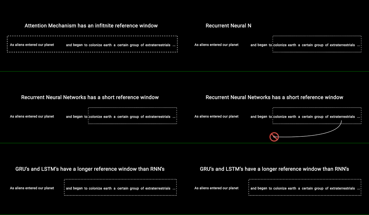
The attention mechanism “describes a weighted average of sequence elements with the weights dynamically computed based on input query and elements’ keys” (“Tutorial 6: Transformers and Multi-Head Attention — UvA DL Notebooks v1.1 Documentation”). When considering words in a sentence, it wouldn’t make sense to weigh each word equally because different words in a sentence could have different impacts on the output. For example, a negation at the beginning of a sentence should probably weigh more because it can significantly change a sentence’s meaning. In other words, we want to dynamically decide on which parts of the sentence we want to give more attention to over others.
When translating a sentence, we typically create some mapping in our heads between different parts of the input sentence and corresponding parts of the output translation. The attention mechanism is the vehicle by which a neural network can learn these mappings via gradient descent and backpropagation. The amount of “attention” is quantified by dynamically learned weights and thus the output of the attention mechanism is usually formed as an attention weighted average. At every time step, we want to dynamically calculate how much attention should be given to the other time steps (before and after). Each time step has a feature vector and the current time step’s feature vector serves as the query (keyword) against which every other timestep’s feature vector (key) is ranked on relevance using a scoring function. The output of these scores is normalized to construct attention weights at that timestep.
In other words, to calculate attention with a query, you compare the query with the keys and get scores/weights for the values. For every word, there is one key and one value vector; the query is compared to all keys with a score function (e.g., a dot product) to determine the weights and the value vectors of all words are averaged via the attention weights (“Tutorial 6: Transformers and Multi-Head Attention — UvA DL Notebooks v1.1 Documentation”).

Self-Attention & Multi-head Attention
The specific attention mechanism used in Transformers is called self-attention. The main idea behind this is the scaled dot product attention, which allows any element in sequence to attend to any other while still being computationally efficient. “Given a query matrix, key matrix, and value matrix, the output is a weighted sum of the value vectors, where the weight assigned to each value slot is determined by the dot-product of the query with the corresponding key” (Weng, Lilian, “The Transformer Family”).
In figure 10 below, the matrix multiplication QK^T computes the dot product for every pair of queries and keys. Each row of the resulting matrix “represents the attention logits for a specific element i to all other elements in the sequence” (“Tutorial 6: Transformers and Multi-Head Attention — UvA DL Notebooks v1.1 Documentation”). On these, a softmax is applied and multiplied with the value vector to get a weighted mean — where the weights are determined by attention. The scaling factor of 1/sqrt(dk) is used to maintain an appropriate variance of attention values after initialization (if not done, the gradients through the softmax will saturate to 1 for one random element and 0 to others — preventing parameters from learning). Thus, the scaled dot product attention allows a neural network to attend over a sequence.

Because we want to consider the multiple different channels a sequence element wants to attend to, the attention mechanism was extended to multiple heads (multiple query-key-value combinations on the same features). Rather than computing the attention once, the multi-head mechanism splits the inputs into chunks and computes the scaled dot-product attention over these subspaces in parallel (Weng, Lilian, “The Transformer Family”). In other words, given a query, key, and value matrix, we can compute sub-queries, sub-keys, and sub-values that all pass through the scaled dot product attention independently and eventually concatenate (and linearly transform to the expected dimensions). Previously, we were computing a single set of attention weights; however, with multi-head attention, we can incorporate multiple perspectives for the task(s) at hand. This is shown in figure 11 below.

If we switch two input elements in the sequence in multi-head attention, the output is exactly the same (this is called permutation-equivariance). While this illustrates that the input is looked at as a set of elements rather than a sequence, what happens in cases where the order of the input is important? To address this, the position should be encoded in the input features. The positional encoding provides order information to the model (a trick with sine and cosine functions to provide the position of each vector to the network).
Transformers
The Transformer model has an encoder-decoder architecture and was originally designed for machine translation. The encoder is responsible for taking an input sentence and generating an attention-based representation; the decoder takes this representation and step-by-step creates a single output, attending over the encoded information. At a high level, this is also how a transformer can be used to generate text given an initial text sequence (shown below).

The first step in the Transformer model is feeding the input to a word embedding layer, which is like a lookup table with learned vector representations of each word. Each word is mapped to a vector with values to represent that word.
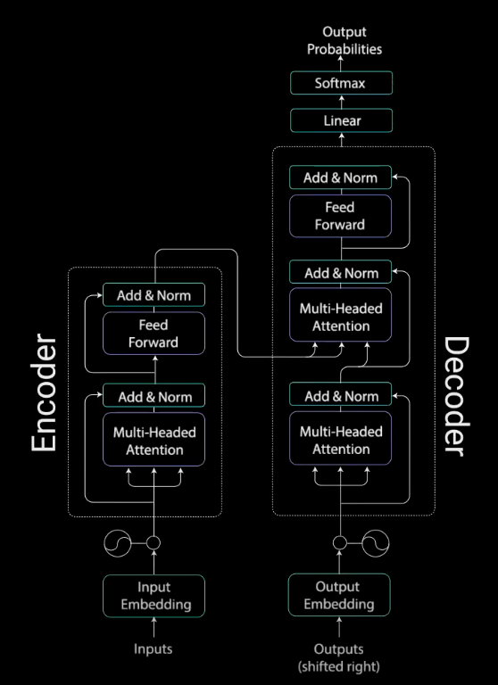
Next, positional information is injected into the embeddings via positional encoding. The next step involves the encoder layer, which maps all input sequences to an abstract continuous representation with the learned information for the sequence. It consists first of a multi-headed attention block. The multi-headed output vector is combined with the original positional input embedding (residual connection) and the output of this goes through layer normalization. Residual connections are important to (1) enable a smooth gradient flow through the deep model and (2) keep information about the original sequence (as the info on input features, which holds the positional info, would be lost after the first attention layer were residual connections removed).
The normalized residual output gets projected through a pointwise feed-forward network for further processing (i.e., linear layers with a ReLU activation in between). The output is added again to the input of the pointwise feed-forward network and further normalized. The idea is that residual connections help the network train by allowing gradients to flow through networks directly. Layer normalization stabilizes the network and reduces the training time.
All these operations are to encode the input to a continuous representation with attention information, which helps the decoder focus on appropriate words in the input when decoding. The encoder can be stacked multiple times, which can be used to further encode the information, where each layer has the opportunity to learn different attention representations. This possibly boosts the predictive power of the transformer network.
The decoder’s job is to generate text sequences. It has a similar sub-layer as the encoder (two multi-headed attention layers, a pointwise feed-forward layer, residual connections, and layer normalization). Decoders act similar to the layers in the encoder, but each multi-headed attention layer has a different job. The decoder is capped off with a linear layer that acts as a classifier and a softmax to get the word probabilities. The decoder is autoregressive. An autoregressive model is a feed-forward model which predicts future values from past values. The decoder begins with a start token and takes in a list of previous outputs as inputs. It also takes the encoder’s outputs that contain attention information from the inputs. When the decoder generates a token as an output, it stops decoding.
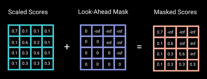
The decoder begins with the input going through an embedding layer and positional encoding layer to get positional embeddings. These embeddings get fed into the first multi-head attention layer, which computes the attention scores for the decoder’s input. Because the decoder is autoregressive and generates the sequence word by word, it must be prevented from conditioning to future tokens. In other words, if you are computing attention scores on the word “am” in the sentence “I am fine,” you shouldn’t have access to the word “fine” because it is a future word that was generated after. The word “am” should only have access to itself and the word(s) before it.
In order to prevent computing attention scores for future words, a method called masking is used. The mask is a matrix that is the same size as the attention scores but filled with the values of 0’s and negative infinity. When the mask is added to scaled attention scores, a matrix of scores is obtained, where the top right triangle is filled with negative infinities. Once you take the softmax of the masked scores, the negative infinities are zeroed out, leaving zero attention scores for future tokens (so no focus is put on these words). A look-ahead mask is applied before calculating the softmax and after scaling the scores. Masking is the only difference in how attention scores are calculated in the first multi-headed attention layer. This layer has multiple heads that the mask is being applied to, before getting concatenated and fed through a linear layer for further processing. The output of the first multi-headed attention is a masked output vector with information on how the model should attend to the decoder’s input (Phi, Michael. “Illustrated Guide to Transformers- Step by Step Explanation”).
The second multi-headed attention layer’s encoder’s outputs are the queries and keys and the first multi-headed attention layer’s outputs are the values. This process matches the encoder’s input to the decoder’s input, allowing the decoder to decide which encoder input is relevant for focus. The output of the second multi-headed attention goes through a pointwise feedforward layer for further processing. The output of this final pointwise feedforward layer goes through a final linear layer, which acts as a classifier (that’s as big as the number of classes present). The output of the classifier then gets fed into a softmax layer, which will produce probability scores between 0 and 1. We take the index of the highest probability score, which equals the predicted word.
The decoder then takes the output, adds it to the list of decoder inputs, and continues decoding again until a token is predicted. The highest probability prediction is the final class that is assigned to the end token.
The decoder can also be stacked (N layers high), where each layer takes in inputs from the encoder and the layers before it. By stacking the layers, the model can learn to extract and focus on different combinations of attention from its attention heads, possibly boosting prediction power.
If you want an easier way to absorb this information, I suggest this video.
Improvements to the Base Transformer Architecture
While vanilla transformers offered a huge improvement over RNN-based seq2seq models, they had a few limitations. The vanilla transformer’s attention mechanism can only deal with fixed-length text strings; the text has to be split into a certain number of segments or chunks before being fed into the system as input. This chunking of text causes context fragmentation (i.e., if a sentence is split from the middle, then a significant amount of context is lost: there’s no consideration for semantic boundaries). Information cannot flow across separated fixed-length segments.
To address context segmentation, the Transformer-XL model was proposed in 2019. It reuses hidden states between segments and uses a new positional encoding for reused states. This enables modeling longer-term dependencies as the information can flow from one segment to the next (Joshi, “Transformers In NLP | State-Of-The-Art-Models”). In the original transformer model, representations from previous segments are computed from scratch during the evaluation phase. Here, computation speed increases because the representations can be reused.
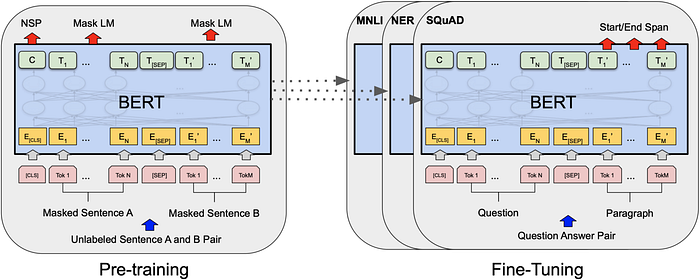
One of the biggest challenges in NLP is the lack of enough training data: deep learning models usually require large amounts of data (millions or billions of annotated training examples). To bridge this data gap, “researchers have developed various techniques for training general-purpose language representation models using the enormous piles of unannotated text on the web” (Khalid, “BERT Explained”). This is known as pre-training. These general-purpose pre-trained models can then be “fine-tuned” on smaller, task-specific datasets and result in performance improvements over training on these task-specific datasets from scratch.
BERT (bidirectional encoder representations from transformers) was a language representation model that uses pre-training and fine-tuning to create state-of-the-art models for a wide range of tasks. If we were to fine-tune BERT for a specific task, we could just add a single layer on top of the core model. This greatly enhanced the ability to conduct transfer learning (“a deep learning model trained on a large dataset [pre-trained model] is used to perform similar tasks on another dataset”) in NLP (Joshi, “Transformers In NLP | State-Of-The-Art-Models”). As BERT’s authors put it, “[BERT] is designed to pre-train deep bidirectional representations from unlabeled text by jointly conditioning on both left and right context… [BERT] can be fine-tuned with just one additional output layer to create state-of-the-art models” (Devlin et al., “BERT”). If curious, please see the paper for more information.
Transformers were a huge step forward for the NLP community and led to many state-of-the-art NLP frameworks like BERT, RoBERTa, and Transformer-XL (which are but a few examples of the numerous frameworks and architectures that are built off or improve vanilla transformers). In my next post, I will introduce Adapters, which are a compact and extensible transfer learning method for NLP that builds off the concepts presented in this post.
Conclusion
There is a lot of exciting work happening in the NLP space at the moment! This article provides a glimpse at previous frameworks that contemporary architectures build off and explains why they were introduced. To recap:
- We briefly summarized what neural networks are and why Recurrent Neural Networks (RNNs) were introduced.
- We described the RNN architecture and challenges associated with deep neural network architectures.
- We provided the impetus for long short-term memory networks (LSTMs) and how memory works in an NLP context.
- We discussed the attention mechanism, self-attention, and multi-head attention as well as why attention matters in an NLP context.
- Finally, we discussed the transformer architecture and improvements to it.
References & Works Cited
I’d like to thank Mohamad Nasr-Azadani (also on Medium!) for his mentorship and guidance as I conducted NLP research and for proofreading my work.
“5 Open Problems in NLP.” Accessed July 6, 2021. https://deeps.site/blog/2019/09/09/nlp-problems//.
Pathmind. “A Beginner’s Guide to LSTMs and Recurrent Neural Networks.” Accessed July 6, 2021. http://wiki.pathmind.com/lstm.
Adaloglou, Nikolas. “Intuitive Explanation of Skip Connections in Deep Learning.” AI Summer, March 23, 2020. https://theaisummer.com/skip-connections/.
“AdapterHub — Adapting Transformers with AdapterHub.” Accessed July 6, 2021. https://adapterhub.ml/blog/2020/11/adapting-transformers-with-adapterhub/.
Analytics Vidhya. “Attention Mechanism In Deep Learning | Attention Model Keras,” November 20, 2019. https://www.analyticsvidhya.com/blog/2019/11/comprehensive-guide-attention-mechanism-deep-learning/.
Brownlee, Jason. “A Gentle Introduction to Backpropagation Through Time.” Machine Learning Mastery (blog), June 22, 2017. https://machinelearningmastery.com/gentle-introduction-backpropagation-time/.
Chapter 7 Transfer Learning for NLP I | Modern Approaches in Natural Language Processing. Accessed August 30, 2021. https://compstat-lmu.github.io/seminar_nlp_ss20/transfer-learning-for-nlp-i.html.
CodeEmporium. Transformer Neural Networks — EXPLAINED! (Attention Is All You Need). Accessed July 6, 2021. https://www.youtube.com/watch?v=TQQlZhbC5ps.
“CS 230 — Recurrent Neural Networks Cheatsheet.” Accessed July 6, 2021. https://stanford.edu/~shervine/teaching/cs-230/cheatsheet-recurrent-neural-networks.
Devlin, Jacob, Ming-Wei Chang, Kenton Lee, and Kristina Toutanova. “BERT: Pre-Training of Deep Bidirectional Transformers for Language Understanding.” ArXiv:1810.04805 [Cs], May 24, 2019. http://arxiv.org/abs/1810.04805.
Elvis. “Adapters: A Compact and Extensible Transfer Learning Method for NLP.” Medium, June 23, 2019. https://medium.com/dair-ai/adapters-a-compact-and-extensible-transfer-learning-method-for-nlp-6d18c2399f62.
Gupta, Tushar. “Deep Learning: Feedforward Neural Network.” Medium, December 16, 2018. https://towardsdatascience.com/deep-learning-feedforward-neural-network-26a6705dbdc7.
Ho, George. “Autoregressive Models in Deep Learning — A Brief Survey.” Eigenfoo, March 9, 2019. https://eigenfoo.xyz/deep-autoregressive-models/.
Joshi, Prateek. “Transformers In NLP | State-Of-The-Art-Models.” Analytics Vidhya (blog), June 19, 2019. https://www.analyticsvidhya.com/blog/2019/06/understanding-transformers-nlp-state-of-the-art-models/.
Khalid, Samia. “BERT Explained: A Complete Guide with Theory and Tutorial.” Towards Machine Learning (blog), September 17, 2019. https://towardsml.com/2019/09/17/bert-explained-a-complete-guide-with-theory-and-tutorial/.
Or, Barak. “The Exploding and Vanishing Gradients Problem in Time Series.” Medium, October 22, 2020. https://towardsdatascience.com/the-exploding-and-vanishing-gradients-problem-in-time-series-6b87d558d22.
Phi, Michael. “Illustrated Guide to Transformers- Step by Step Explanation.” Medium, June 28, 2020. https://towardsdatascience.com/illustrated-guide-to-transformers-step-by-step-explanation-f74876522bc0.
Sciforce. “Biggest Open Problems in Natural Language Processing.” Medium, February 5, 2020. https://medium.com/sciforce/biggest-open-problems-in-natural-language-processing-7eb101ccfc9.
Turc, Iulia. “Unsolved Problems in Natural Language Datasets.” Medium, August 26, 2020. https://towardsdatascience.com/unsolved-problems-in-natural-language-datasets-2b09ab37e94c.
“What Is a Projection Layer in the Context of Neural Networks? — Intellipaat Community.” Accessed August 30, 2021. https://intellipaat.com/community/1864/what-is-a-projection-layer-in-the-context-of-neural-networks.
“What Is the Downside of Using LSTM versus RNN in Deep Learning? — Quora.” Accessed July 6, 2021. https://www.quora.com/What-is-the-downside-of-using-LSTM-versus-RNN-in-Deep-Learning.
“4. Recurrent Neural Networks — Neural Networks and Deep Learning [Book].” Accessed November 18, 2021. https://www.oreilly.com/library/view/neural-networks-and/9781492037354/ch04.html.
Pere, Christophe. “What Are Loss Functions?” Medium, June 18, 2020. https://towardsdatascience.com/what-is-loss-function-1e2605aeb904.
Stack Overflow. “Backpropagation — What Are Forward and Backward Passes in Neural Networks?” Accessed November 23, 2021. https://stackoverflow.com/questions/36740533/what-are-forward-and-backward-passes-in-neural-networks.
Artificial Intelligence Stack Exchange. “Recurrent Neural Networks — What Exactly Is a Hidden State in an LSTM and RNN?” Accessed November 23, 2021. https://ai.stackexchange.com/questions/16133/what-exactly-is-a-hidden-state-in-an-lstm-and-rnn.
Silva, Thalles. “Machine Learning 101: An Intuitive Introduction to Gradient Descent.” Medium, August 15, 2019. https://towardsdatascience.com/machine-learning-101-an-intuitive-introduction-to-gradient-descent-366b77b52645.
DEV Community. “Let’s Pay Some Attention!” Accessed November 23, 2021. https://dev.to/shambhavicodes/let-s-pay-some-attention-33d0.
Kirill Eremenko. “Deep Learning A-ZTM: Recurrent Neural Networks (RNN) — The Vanishing G….” 16:13:47 UTC. https://www.slideshare.net/KirillEremenko/deep-learning-az-recurrent-neural-networks-rnn-the-vanishing-gradient-problem.
Imgur. “RNN vs LSTM: Vanishing Gradients — GIF.” Imgur. Accessed December 6, 2021. https://imgur.com/gallery/vaNahKE.
Quora. “What Is the Downside of Using LSTM versus RNN in Deep Learning?” Accessed December 6, 2021. https://www.quora.com/What-is-the-downside-of-using-LSTM-versus-RNN-in-Deep-Learning.
“Understanding LSTM Networks — Colah’s Blog.” Accessed December 6, 2021. https://colah.github.io/posts/2015-08-Understanding-LSTMs/.
Brownlee, Jason. “What Are Word Embeddings for Text?” Machine Learning Mastery (blog), October 10, 2017. https://machinelearningmastery.com/what-are-word-embeddings/.
Doshi, Ketan. “Transformers Explained Visually (Part 1): Overview of Functionality.” Medium, June 3, 2021. https://towardsdatascience.com/transformers-explained-visually-part-1-overview-of-functionality-95a6dd460452.
Alammar, Jay. “The Illustrated Transformer.” Accessed December 21, 2021. https://jalammar.github.io/illustrated-transformer/.
Wei, Jerry. “BERT: Why It’s Been Revolutionizing NLP.” Medium, September 2, 2020. https://towardsdatascience.com/bert-why-its-been-revolutionizing-nlp-5d1bcae76a13.
English Language Learners Stack Exchange. “Grammar — Changing the Word Order Changes the Meaning?” Accessed December 23, 2021. https://ell.stackexchange.com/questions/47172/changing-the-word-order-changes-the-meaning.
“Tutorial 6: Transformers and Multi-Head Attention — UvA DL Notebooks v1.1 Documentation.” Accessed January 2, 2022. https://uvadlc-notebooks.readthedocs.io/en/latest/tutorial_notebooks/tutorial6/Transformers_and_MHAttention.html.
Weng, Lilian. “The Transformer Family.” Lil’Log, April 7, 2020. https://lilianweng.github.io/2020/04/07/the-transformer-family.html.
